plot

visualize fits from an mpm object

# S3 method for mpm_df
plot(
  x,
  y = NULL,
  se = FALSE,
  pages = 0,
  ncol = 1,
  ask = TRUE,
  pal = "Plasma",
  rev = FALSE,
  ...
)

Arguments

x

a aniMotum mpm fit object with class mpm_df

y

optional ssm fit object with class ssm_df corresponding to x. If absent, 1-d plots of gamma_t time series are rendered otherwise, 2-d track plots with locations coloured by `gamma_t`` are rendered.

se

logical (default = FALSE); should points be scaled by gamma_t uncertainty (ignored if y is not supplied)

pages

plots of all individuals on a single page (pages = 1; default) or each individual on a separate page (pages = 0)

ncol

number of columns to use for faceting. Default is ncol = 1 but this may be increased for multi-individual objects. Ignored if pages = 0

ask

logical; if TRUE (default) user is asked for input before each plot is rendered. set to FALSE to return ggplot objects

pal

grDevices::hcl.colors palette to use (default: "Plasma"; see grDevices::hcl.pals for options)

rev

reverse colour palette (logical)

...

additional arguments to be ignored

Value

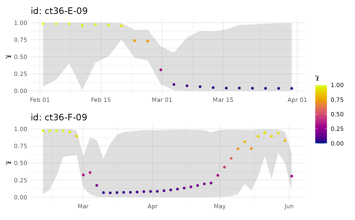
a ggplot object with either: 1-d time series of gamma_t estimates (if y not provided), with estimation uncertainty ribbons (95 % CI's); or 2-d track plots (if y provided) coloured by gamma_t, with smaller points having greater uncertainty (size is proportional to SE^-2, if se = TRUE). Plots can be rendered all on a single page (pages = 1) or on separate pages.

Examples

# generate a ssm fit object (call is for speed only)
xs <- fit_ssm(sese2, spdf=FALSE, model = "rw", time.step=72, control = ssm_control(verbose = 0))
#> 
#> 

# fit mpm to ssm fits
xm <- fit_mpm(xs, model = "jmpm")
#> fitting jmpm...
#> 
 pars:   0 0 0      
 pars:   -0.63038 -0.77416 0.05745      
 pars:   -0.21961 -0.90381 0.95993      
 pars:   0.1024 -0.34798 0.19353      
 pars:   -0.12912 -0.74761 0.74455      
 pars:   -0.17853 -0.8329 0.86216      
 pars:   -0.23363 -0.801 0.86597      
 pars:   -0.27635 -0.61987 0.76146      
 pars:   -0.40458 -0.79384 0.62587      
 pars:   -0.36412 -0.6719 0.40545      
 pars:   -0.38583 -0.70377 0.60569      
 pars:   -0.43697 -0.67572 0.577      
 pars:   -0.38583 -0.70377 0.60569      

# plot 1-D mp timeseries on 1 page
plot(xm, pages = 1)