Mapping

map()

aniMotum provides a flexible map function for mapping SSM-estimated tracks along with options for including their confidence ellipses, observed locations, track lines, and behavioural estimates. Default choices are made based on the model fit object being mapped but these can be overridden via the aes argument and the aes_lst() function.

Map an SSM fit to data, using default settings

se2 <- subset(sese, id %in% unique(id)[1:2])
fit <- fit_ssm(se2, 
               model = "mp", 
               time.step = 24, 
               control = ssm_control(verbose = 0))

map(fit, what = "predicted")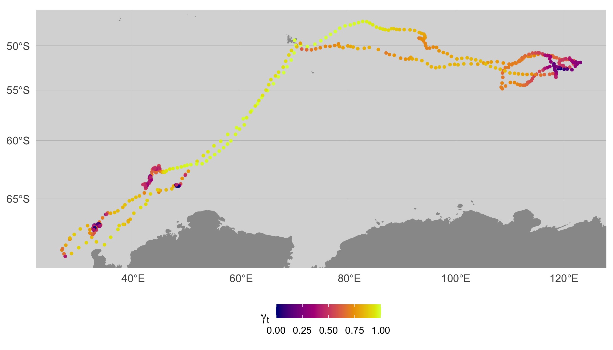

Here, SSM-predicted locations are coloured by the estimated move persistence index ($\gamma_t$). To aid visualisation of high and low move persistence regions along each track, the $\gamma_t$ estimates are normalised separately for each track to span the interval 0,1. This can be turned off with normalise = FALSE, or applied to the group of tracks with group = TRUE.

By default, map() will try to use rnaturalearth::ne_countries(scale = 10) high-resolution land polygon data if the rnaturalearthhires data package is installed. If not, the default will be dropped to the coarser scale=50. The rnaturalearthhires package can be installed via: install.packages("rnaturalearthhires", repos = "https://ropensci.r-universe.dev") or remotes::install_github("ropensci/rnaturalearthhires"). Alternatively, if the ggpstial and rosm packages are installed, users may specify any of the available tile map layers returned by rosm::osm.types() via the map_type argument. When specifying a map_type, map will take any additional arguments to ggspatial::annotation_map_tile() for finer control; zoom and progress are used here.

map(fit, what = "predicted", map_type = "cartodark", zoom = 4, progress = "none")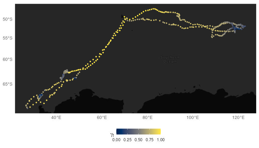

Control track components

We can add and remove certain track components by using the aes argument and aes_lst() function. Here, the observed locations (orange triangles) and track lines have been turned on and the move persistence index has been turned off.

my.aes <- aes_lst(obs=TRUE, line=TRUE, mp=FALSE)

map(fit, what = "p", aes = my.aes)

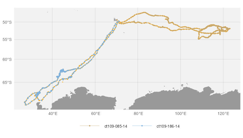
Note that when turning off the move persistence index, tracks are automatically given unique colours. This can be turned off by using by.id = FALSE.

Additional control over mapping aesthetics can be gained by viewing and editing the my.aes$df data.frame created by aes_lst(). We can subset components and assign new values as needed, here we change the observation colour and shape from orange triangles to firebrick diamonds. We also set by.id = FALSE so all tracks are displayed in a unique colour (default is “dodgerblue”).

my.aes$df

my.aes$df$col[4] <- "firebrick"
my.aes$df$shape[4] <- 18

map(fit, 
    what = "p", 
    aes = my.aes, 
    by.id = FALSE)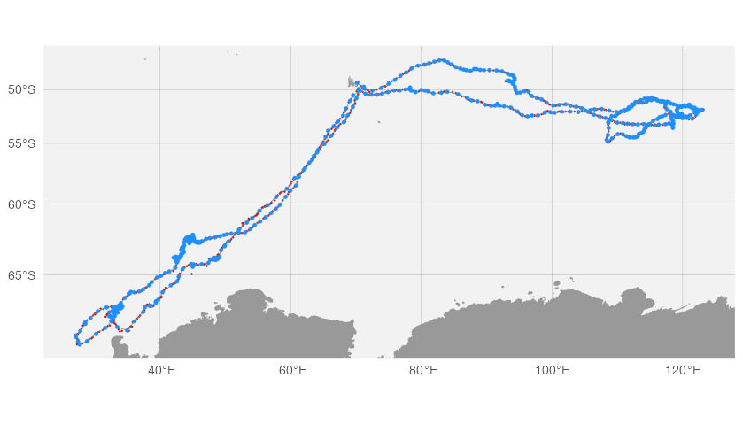

Alternatively, we can colour estimated locations by their date to better see how tracks evolve over time.

map(fit, 
    what = "p", 
    aes = aes_lst(mp=FALSE, conf=FALSE), 
    by.date = TRUE, 
    by.id=FALSE)

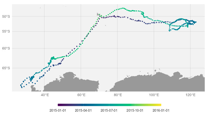
If you don’t like the default colour palettes, these can be changed by modifying the default aes object. Here, the hcl.colors() function is used to specify a new colour palette for displaying date-along-track.

map(fit, 
    what = "p", 
    aes = aes_lst(mp=FALSE, 
                  conf=FALSE, 
                  date_pal = hcl.colors(n=100, "Plasma")), 
    by.date = TRUE, by.id=FALSE)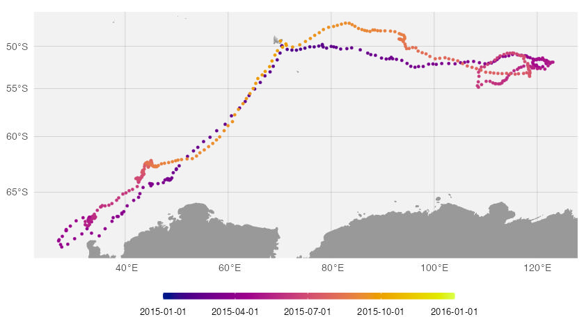

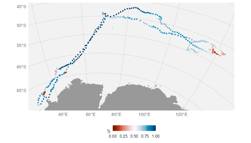
And similarly for displaying move persistence.

map(fit, 
    what = "p", 
    aes = aes_lst(mp_pal = hcl.colors(n=100, "RdBu")))

Change projection

Often choosing an appropriate map projection can provide a more meaningful view of the tracks, especially for animals that make very broad-scale movements, such as the southern elephant seals displayed here. This can be done easily by providing a valid proj4string for the Coordinate Reference System. Here, we project the tracks onto a polar stereographic grid with longitude centered on 68^o East, Iles Kerguelen.

map(fit, 
    what = "p", 
    aes = aes_lst(mp_pal = hcl.colors(n=100, "RdBu")), 
    crs = "+proj=stere +lon_0=68 +datum=WGS84 +units=km")