plot

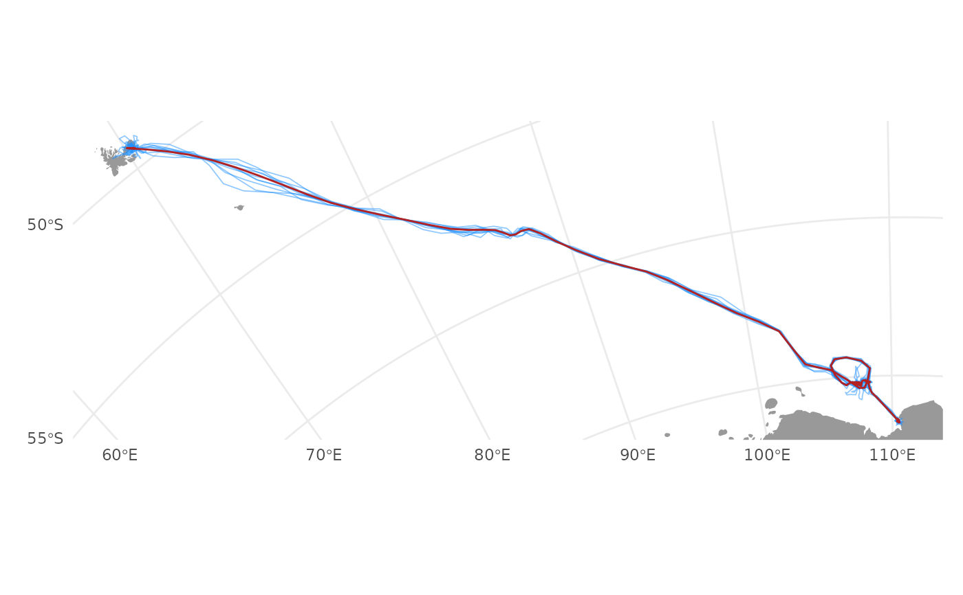
visualize tracks simulated from a aniMotum model fit

# S3 method for sim_post
plot(
  x,
  type = c("lines", "points", "both"),
  zoom = TRUE,
  ncol = 1,
  hires = TRUE,
  ortho = TRUE,
  alpha = 0.5,
  ...
)

Arguments

x

a aniMotum simulation data.frame with class sim_fit

type

plots tracks as "line", "points" or "both" (default).

zoom

logical; should map extent be defined by track extent (TRUE; default) or should global map be drawn (FALSE).

ncol

number of columns to arrange multiple plots

hires

logical; use high-resolution coastline data. Attempts to use high-res coastline data via rnaturalearth::ne_countries with scale = 10, if the rnaturalearthhires data package is installed. If not, then rnaturalearth::ne_countries with scale = 50 data are used.

ortho

logical; use an orthographic projection centered on the track starting location(s) (TRUE; default). An orthographic projection may be optimal for high latitude tracks and/or tracks that traverse long distances. If FALSE then a global Mercator projection is used.

alpha

opacity of simulated track points/lines. Lower opacity can ease visualization when multiple simulated overlap one another.

...

additional arguments to be ignored

Value

Plots of posterior simulated tracks.

Examples

fit <- fit_ssm(ellie, model = "crw", time.step = 24)
#> fitting crw SSM to 1 tracks...
#> 
 pars:   1 1 0 -2.91153      
 pars:   0.38512 0.37191 -0.01692 -3.38813      
 pars:   -1.4595 -1.51236 -0.06769 -4.81792      
 pars:   -2.20058 -2.24383 -0.11527 -4.95732      
 pars:   -0.38346 -0.4056 -0.04615 -3.85456      
 pars:   -1.23664 -1.20844 -0.10327 -3.65984      
 pars:   -2.25711 -2.16871 -0.17159 -3.42693      
 pars:   -3.07868 -3.34599 -0.26131 -1.24778      
 pars:   -4.46619 -1.62751 -0.49092 0.12579      
 pars:   -3.18442 -2.86245 -0.30197 -0.80151      
 pars:   -3.40955 -3.30581 -0.49919 -0.40195      
 pars:   -3.06893 -3.16418 -1.05454 -0.36585      
 pars:   -3.5513 -2.81435 -1.34642 -0.44033      
 pars:   -3.30092 -3.01944 -1.10395 -0.39263      
 pars:   -3.27833 -3.03821 -1.38152 -0.39631      
 pars:   -3.23173 -2.97174 -2.21731 -0.40477      
 pars:   -3.28771 -3.08271 -5.28966 -0.34232      
 pars:   -3.30222 -3.07091 -5.31779 -0.38305      
 pars:   -3.30222 -3.07091 -5.31779 -0.38305      
psim <- sim_post(fit, what = "p", reps = 10)
plot(psim, type = "lines")