simulate animal tracks from a ssm fit — sim

simulate from the rw or crw process models to generate either a set of x,y or lon,lat coordinates from a ssm fit with length equal to the number of observations used in the SSM fit.

sim_fit(
  x,
  what = c("fitted", "predicted"),
  reps = 1,
  start = NULL,
  end = NULL,
  grad = NULL,
  beta = c(-300, -300),
  cpf = FALSE,
  sim_only = FALSE
)

Arguments

x: a ssm fit object with class ssm_df
what: simulate fitted (typically irregular in time) or predicted (typically regular in time) locations
reps: number of replicate tracks to simulate from an ssm model fit object
start: a 2-element vector for the simulated track start location (lon,lat or x,y)
end: a 2-element vector for the simulated track end location (lon,lat or x,y)
grad: a SpatRaster of x- and y-gradients as separate layers (see details)
beta: a 2-element vector of parameters defining the potential function magnitude in x- and y-directions (ignored if is.null(grad), ie. no potential function; see details).
cpf: logical; should simulated tracks return to their start point (ie. a central-place forager)
sim_only: logical, do not include ssm estimated location in output (default is FALSE)

Value

a fG_sim_fit object containing the paths simulated from a ssm fit object

Details

A potential function can be applied to the simulated paths to help avoid locations on land (or in water), using the grad and beta arguments. A coarse-resolution rasterStack of global x- and y-gradients of distance to land are provided. Stronger beta parameters result in stronger land (water) avoidance but may also introduce undesirable/unrealistic artefacts (zig-zags) in the simulated paths. See Brillinger et al. (2012) and vignette("momentuHMM", package = "momentuHMM") for more details on the use of potential functions for simulating constrained animal movements. WARNING: This application of potential functions to constrain simulated paths is experimental, likely to change in future releases, and NOT guaranteed to work enitrely as intended, especially if cpf = TRUE!

References

Brillinger DR, Preisler HK, Ager AA, Kie J (2012) The use of potential functions in modelling animal movement. In: Guttorp P., Brillinger D. (eds) Selected Works of David Brillinger. Selected Works in Probability and Statistics. Springer, New York. pp. 385-409.

Examples

fit <- fit_ssm(ellie, model = "crw", time.step = 24)
#> fitting crw SSM to 1 tracks...
#> 
 pars:   1 1 0 -2.91153      
 pars:   0.38512 0.37191 -0.01692 -3.38813      
 pars:   -1.4595 -1.51236 -0.06769 -4.81792      
 pars:   -2.20058 -2.24383 -0.11527 -4.95732      
 pars:   -0.38346 -0.4056 -0.04615 -3.85456      
 pars:   -1.23664 -1.20844 -0.10327 -3.65984      
 pars:   -2.25711 -2.16871 -0.17159 -3.42693      
 pars:   -3.07868 -3.34599 -0.26131 -1.24778      
 pars:   -4.46619 -1.62751 -0.49092 0.12579      
 pars:   -3.18442 -2.86245 -0.30197 -0.80151      
 pars:   -3.40955 -3.30581 -0.49919 -0.40195      
 pars:   -3.06893 -3.16418 -1.05454 -0.36585      
 pars:   -3.5513 -2.81435 -1.34642 -0.44033      
 pars:   -3.30092 -3.01944 -1.10395 -0.39263      
 pars:   -3.27833 -3.03821 -1.38152 -0.39631      
 pars:   -3.23173 -2.97174 -2.21731 -0.40477      
 pars:   -3.28771 -3.08271 -5.28966 -0.34232      
 pars:   -3.30222 -3.07091 -5.31779 -0.38305      
 pars:   -3.30222 -3.07091 -5.31779 -0.38305      
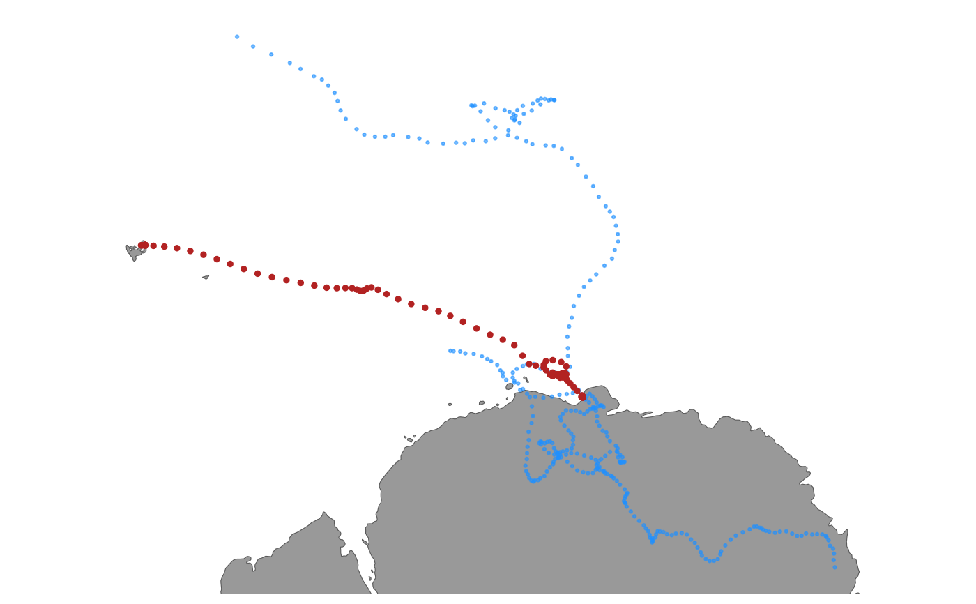
trs <- sim_fit(fit, what = "predicted", reps = 3)
plot(trs)