Filter sim_fit simulations — sim

This function calculates the similarity between the simulations generated by sim_fit and the SSM-estimated path from the ssm fit, and returns a sim_fit object containing the most similar tracks based on a user specified quantile. In this context, similarity is calculated as the sum of normalised differences in net displacement (km) and overall bearing (deg) between the SSM-estimated path and the simulated paths.

sim_filter(trs, keep = 0.25, flag = 2, var = NULL, FUN = "mean", ...)

Arguments

trs: a sim_fit object
keep: the quantile of flag values to retain
flag: the similarity flag method (see details). Ignored if var != NULL.
var: the name(s) of the appended variable(s) to use for similarity calculations. Default is NULL, in which case similarity is calculated based on distance and bearing - e.g., Hazen et al (2017).
FUN: one of the following functions in quotes: mean, median, var, sd, sum, min, or max. Ignored if var = NULL.
...: additional arguments to the specified FUN (e.g., na.rm = TRUE). Ignored if var = NULL.

Value

a sim_fit object containing the filtered paths

Details

flag = 1 will use an index based on Hazen (2017)
flag = 2 (the default) will use a custom index

References

Hazen et al. (2017) WhaleWatch: a dynamic management tool for predicting blue whale density in the California Current J. Appl. Ecol. 54: 1415-1428

Examples

## fit crw model to Argos LS data
fit <- fit_ssm(ellie, model = "crw", time.step = 72)
#> fitting crw SSM to 1 tracks...
#> 
 pars:   1 1 0 -3.35398      
 pars:   0.39011 0.36995 -0.01715 -3.83437      
 pars:   -1.43958 -1.5202 -0.06862 -5.27553      
 pars:   -2.32555 -2.54729 -0.19371 -4.12372      
 pars:   -0.8182 -0.89535 -0.06643 -4.50381      
 pars:   -1.32518 -1.50336 -0.13293 -2.80663      
 pars:   -2.70765 -2.68894 -0.23564 -2.37746      
 pars:   -3.27563 -3.39761 -0.40156 -0.74674      
 pars:   -4.54561 -2.25375 -0.86806 -0.13627      
 pars:   -3.3297 -3.27793 -0.43777 -0.61077      
 pars:   -3.36938 -3.29518 -0.51676 -0.44068      
 pars:   -3.37129 -3.28379 -0.68713 -0.35188      
 pars:   -3.37129 -3.28379 -0.68713 -0.35188      

set.seed(pi)
## generate 5 simulated paths from ssm fit
trs <- sim_fit(fit, what = "predicted", reps = 5)

## filter simulations and keep paths in top 40% of flag values
trs_f <- sim_filter(trs, keep = 0.4, flag = 2)

## compare unfiltered and filtered simulated paths
# \donttest{
plot(trs) | plot(trs_f)

# }
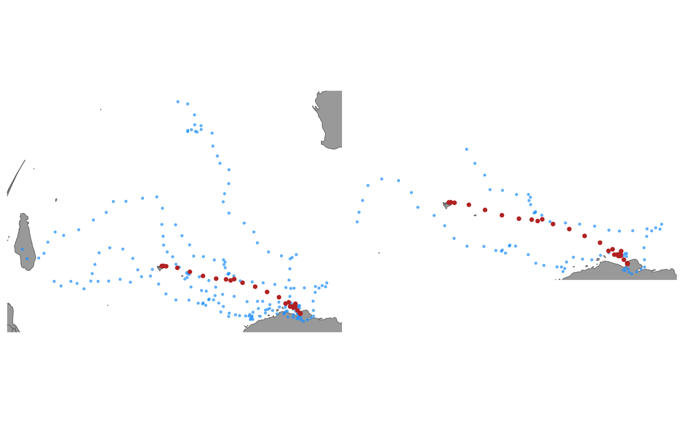